
| project name: |
| decimal numbers: | ||
| exponential numbers: |
The CFLOW solver is a quasi-one-dimensional Finite Volume Method (FVM) solver, which means that flow quantities varies in one direction only and there may be smooth variations in the cross-section area.
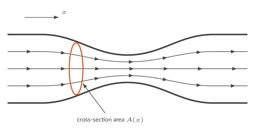
More details can be found here:
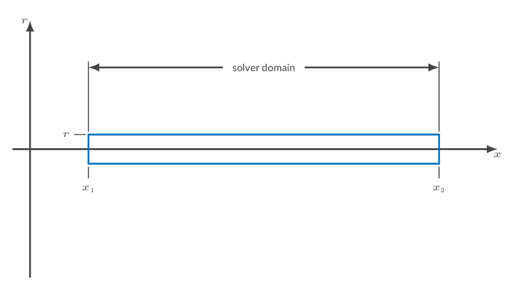
Select a flow domain type from the drop-down list and specify coordinates accordingly. The domain sketch above is updated on domain type change in order to give some guidance on how to specify the requested input.
| pipe type: |
| left end coordinate \((x_1)\): | |||
| right end coordinate \((x_2)\): | |||
| throat coordinate \((x_t)\): | |||
| interface coordinate \((x_i)\): |
Radial coordinates at the requested locations (the number of locations depends on domain type) can be specified as radius, diameter, or cross-section area. Make sure to select the appropriate dimension for your specified input.
| cross-section | \((r_1)\): | \((D_1)\): | \((A_1)\): | |||
| right end cross-section | \((r_2)\): | \((D_2)\): | \((A_2)\): | |||
| throat cross-section | \((r_t)\): | \((D_t)\): | \((A_t)\): |
Spatial discretization is achieved by dividing the computational domain into small elements (cells) and apply the integral form of the continuity, momentum and energy equations to these cells. The result is a system of ordinary differential equations with the cell averages of density, momentum and energy in all cells as degrees of freedom.
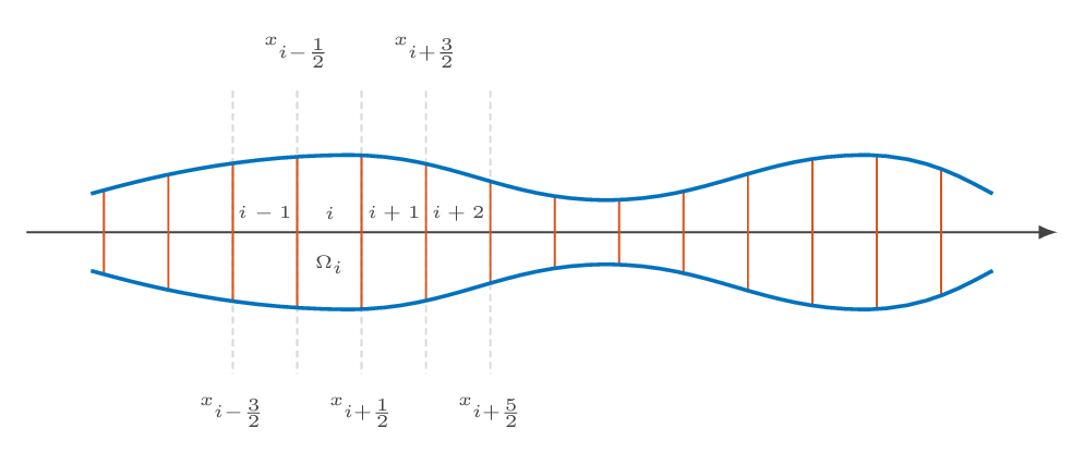
A close-up of cell \(\Omega_i\)
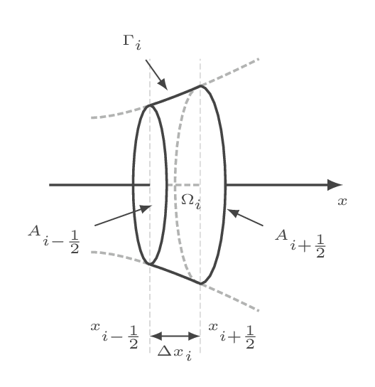
The discretized flow equations for cell \(\Omega_i\)

More details can be found here:
| Quasi-one-dimensional flow | |
| The time-marching technique | (Spatial discretization) |

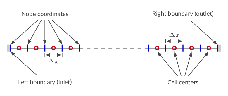
Specify the number of finite-volume cells that should be used to discretize the fluid domain in the flow direction. For some of the domain types (selected in the geometry settings), the number of cells in different flow regions should be specified. Unless the current domain type supports mesh refinement, all cells in the domain will be of equal size, i.e., the length of domain will be divided by the specified number of cells, each with the length \(\Delta x\) (see figure below).
| number of cells: | |||
| number of cells in region 1: | (from inlet to throat) | ||
| number of cells in region 2: | (from throat to shock) | ||
| number of cells in region 3: | (from shock to exit) | ||
The mesh can be refined locally by specifying a cell size smaller than the uniform distribution cell size.
| cell spacing: | |||
| cell spacing: | |||
| cell spacing: | |||
| axial coordinate \((x_l)\): | |||
| cell spacing: | |||
| cell spacing: | |||
Discretizing results in a system of ordinary differential equations including cell-averaged flow quantities (orange), cell face values of flow properties (blue), and, for the quasi-one-dimensional approach, a pressure source term (green). The cell averaged flow quantities in all cells are the degrees of freedom but the face values are not known.


The face values needs to be expressed as a function of the known cell-averaged flow variables.
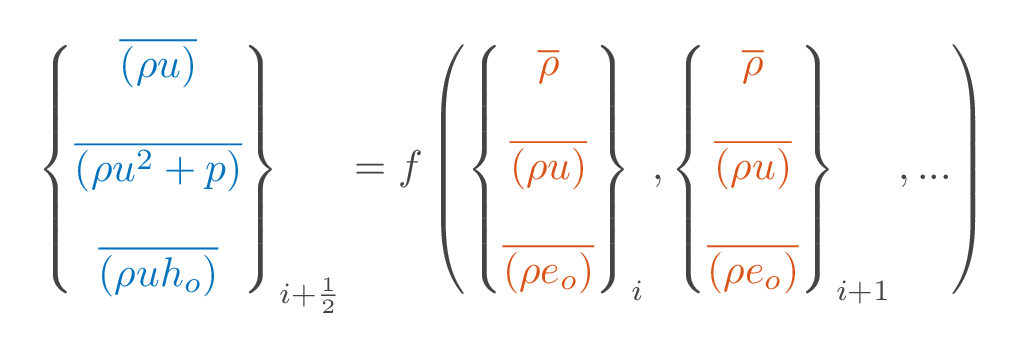
Calculating the cell face value as the average of two neighbouring cells corresponds to a central difference scheme.

In case there are shocks or steep temperature gradients in the flow field, extra artifical damping may need to be used to get the solver stable. Pressure damping is used for problems with shocks (a typical value is 0.5) and density damping is used for problems with steep temperature gradients (a typical value is 2.0). Problems may need either pressure damping or density damping or both. Problems without shocks or steep gradients of temperature do not need damping.
The CFLOW solver uses an explicit three-stage Runge-Kutta time marching technique. This means that, in order for the solver to be stable, information cannot be allowed to travel more than one cell width in one time step. In the schematic representation below, the fastest characteristic (C+ or C-) decides the time step so that the CFL number is equal to one.
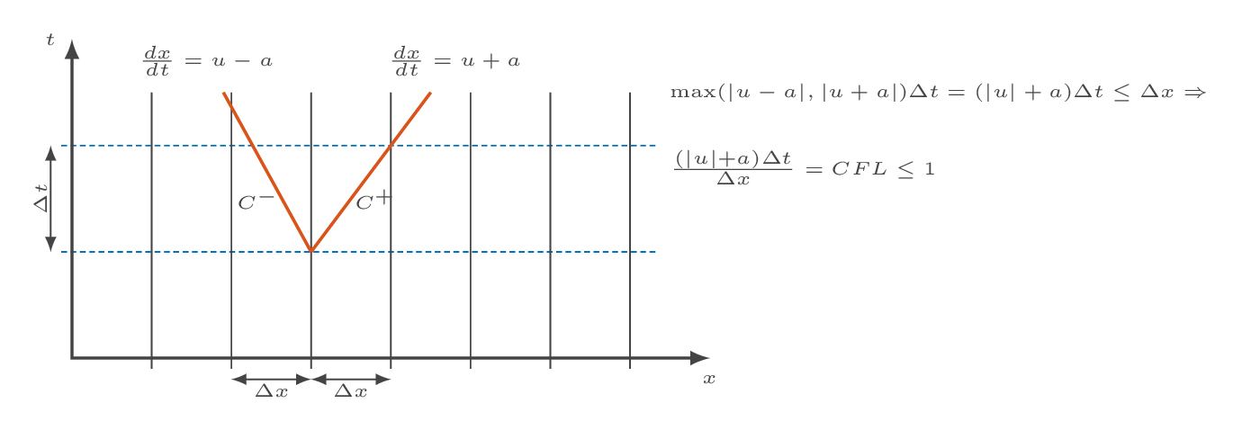
In the CFLOW solver, there are three different time stepping modes:
More details can be found here:
| The time-marching technique | (Spatial discretization & Time stepping) |
Select a numerical scheme. The default alternative (third-order upwind) works fine in most cases
| convective scheme: |
Add extra artificial numerical damping if needed. Only applicable for cases with shocks and/or steep temperature gradients.
| shocks: | (pressure-based damping - typical value: 0.5) | |
| temperature gradients: | (density-based damping - typical value: 2.0) |
Select time stepping mode and specify CFL number or time step size. Read more about the different time stepping modes in the info box above (press the i-button).
| time stepping mode: | ||
| CFL number: | \(CFL=\frac{\Delta t\left(c+\|u\|\right)}{\Delta x}\) | |
| time step: | seconds |
The specified number of time steps will be executed each time the solver is started. If "save old flow data" is set to "yes", the flow field state after each completed "number of iterations" will be stored in the flow data archive available in the postprocessing section. If "save old flow data" is set to "no", only the latest solver flow state will be stored.
| Number of time steps | |
| Save old flow data |
Specify gas properties (ratio of specific heats and gas constant) for the simulated gas. The default values are the gas properties for air \((\gamma=C_p/C_v=1.4,\ R=287)\).
| ratio of specific heats \(\left(\gamma\right)\) | ||||
| gas constant \(\left(R\right)\) |

Specify an initial flow field (start solution) either as constant values (same in all cells) or as a linear distribution from the domain inlet to the domain outlet (not possible for all domain types). If "constant values" is selected, setting the flow conditions at either the domain inlet or the domain outlet as the initial flow state is most often a stable start solution but not always.
For some domain types, different flow regions should be initiated separately. This enables using a discontinuous start solution, which is applicable if, for example, simulating a shock tube.
| initialization mode |
| specified variables | ||||||
| temperature: | ||||||
| density: | ||||||
| axial velocity: | ||||||
| pressure: | ||||||
| specified variables | ||||||
| temperature: | ||||||
| density: | ||||||
| axial velocity: | ||||||
| pressure: | ||||||
If applicable, specify amplitude and wavelength of an acoustic perturbation to be superimposed on the specified initial solution.
| pressure amplitude \(\left(\Delta P\right)\): | ||||||
| wave length \(\left(\lambda\right)\): |
Select a solution from the solution archive to be interpolated into the current mesh. This option can be used if the mesh has been updated and one would like to use an old solution a start solution for a new simulation.
In compressible flow simulations, the boundary conditions are defined based on analysis of characteristics at the boundary.
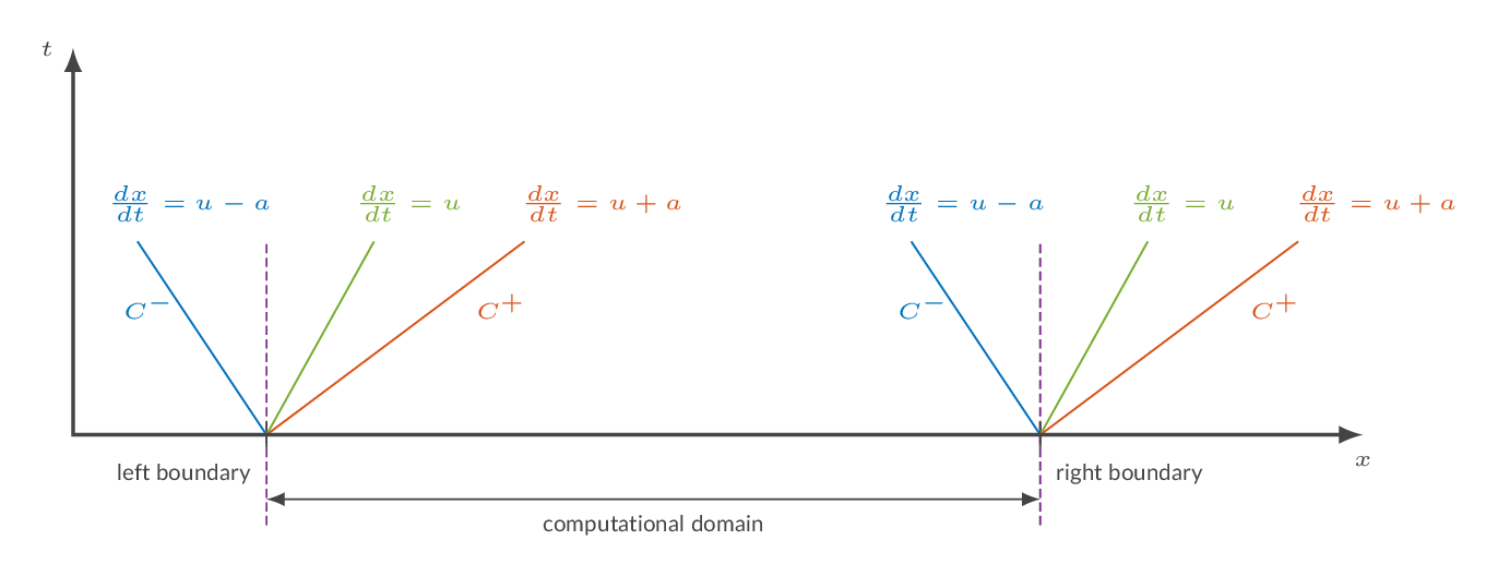
As can be seen from the schematic representation above, there are three characteristics, namely, C+, C-, and advection.
| Characteristic | 1D subsonic inflow (left) | 1D subsonic inflow (right) | |
|---|---|---|---|
| advection | \(\mathbf{v}\cdot\mathbf{n}\) | \((u,0,0)\cdot(-1,0,0)=-u<0\) | \((-u,0,0)\cdot(1,0,0)=-u<0\) |
| \(C^-\) | \(\mathbf{v}\cdot\mathbf{n}-a\) | \(-u-a<0\) | \(-u-a<0\) |
| \(C^+\) | \(\mathbf{v}\cdot\mathbf{n}+a\) | \(-u+a>0\) | \(-u+a>0\) |
| Characteristic | 1D subsonic outflow (left) | 1D subsonic outflow (right) | |
| advection | \(\mathbf{v}\cdot\mathbf{n}\) | \((-u,0,0)\cdot(-1,0,0)=u>0\) | \((u,0,0)\cdot(1,0,0)=u>0\) |
| \(C^-\) | \(\mathbf{v}\cdot\mathbf{n}-a\) | \(u-a<0\) | \(u-a<0\) |
| \(C^+\) | \(\mathbf{v}\cdot\mathbf{n}+a\) | \(u+a>0\) | \(u+a>0\) |
| Characteristic | 1D supersonic inflow (left) | 1D supersonic inflow (right) | |
| advection | \(\mathbf{v}\cdot\mathbf{n}\) | \((u,0,0)\cdot(-1,0,0)=-u<0\) | \((-u,0,0)\cdot(1,0,0)=-u<0\) |
| \(C^-\) | \(\mathbf{v}\cdot\mathbf{n}-a\) | \(-u-a<0\) | \(-u-a<0\) |
| \(C^+\) | \(\mathbf{v}\cdot\mathbf{n}+a\) | \(-u+a<0\) | \(-u+a<0\) |
| Characteristic | 1D supersonic outflow (left) | 1D supersonic outflow (right) | |
| advection | \(\mathbf{v}\cdot\mathbf{n}\) | \((-u,0,0)\cdot(-1,0,0)=u>0\) | \((u,0,0)\cdot(1,0,0)=u>0\) |
| \(C^-\) | \(\mathbf{v}\cdot\mathbf{n}-a\) | \(u-a>0\) | \(u-a>0\) |
| \(C^+\) | \(\mathbf{v}\cdot\mathbf{n}+a\) | \(u+a>0\) | \(u+a>0\) |
| boundary type | ingoing/outgoing characteristics | example of specified variables |
|---|---|---|
| 1D subsonic inflow | 2/1 (specify two variables) | \(p_o,\ T_o\) |
| 1D subsonic outflow | 1/2 (specify one variable) | \(p\) |
| 1D supersonic inflow | 3/0 (specify all flow variables) | \(\rho,\ u,\ p\) |
| 1D supersonic outflow | 0/3 (specify nothing) | - |
In addition to the boundary condition listed above, CFLOW has a non-reflective boundary condition in which a characteristic analysis is done in each evaluation. For the non-reflective boundary condition, boundary values of \(\rho\), \(u\), and \(p\) should be specified.
There is also a periodic boundary condition and a solid wall boundary condition. In the periodic boundary condition, the inlet and outlet will be coupled, i.e., what exits the outlet will enter the inlet and the other way around.
More details can be found here:
| The time-marching technique | (Boundary conditions) |


Specify boundary condition type for the left and right end boundaries and fill in requested flow field data. Information about the different boundary conditions can be found in the info box above (press the i-button).
| boundary condition type | ||||||
| density \(\left(\rho\right)\): | ||||||
| velocity \(\left(u\right)\): | ||||||
| pressure \(\left(P\right)\): | ||||||
| total pressure \(\left(P_o\right)\): | ||||||
| total temperature \(\left(T_o\right)\): | ||||||
| boundary condition type | ||||||
| density \(\left(\rho\right)\): | ||||||
| velocity \(\left(u\right)\): | ||||||
| pressure \(\left(P\right)\): | ||||||
| total pressure \(\left(P_o\right)\): | ||||||
| total temperature \(\left(T_o\right)\): | ||||||
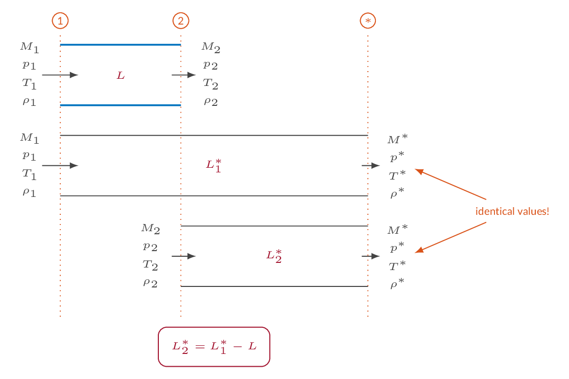
When friction is added to a one-dimensional flow, the Mach number will approach 1.0 (sonic flow). For an initially subsonic flow, the Mach number will increase until sonic conditions are reached and for an initially supersonic flow, added friction will reduce the Mach number until sonic conditions are reached. In the calculations below, friction is introduced using a constant friction factor, which means that the amount of friction added is a linear function of pipe length. The length for which sonic conditions are reached is denoted \(L^*\) and starred flow properties are flow properties at sonic conditions. The starred flow quantities are constants in a specific flow. When sonic conditions are reached, the flow is choked and more friction (pipe length) cannot be added without changing the upstream flow conditions.
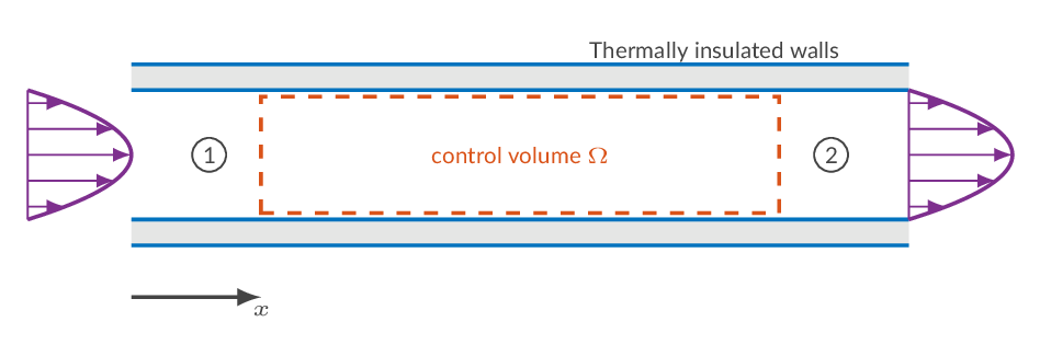
A typical problem is the two-station problem i.e., a problem where flow properties are known at one location in the flow and the flow properties in an upstream or downstream location should be calculated. This is done using the starred quantities as a reference state. The starred flow quantities are calculated based on the flow quantities in station 1. As the starred quantities are constants, they can be used together with the added friction to calculate the flow properties in station 2.
| flow property | subsonic flow with friction | supersonic flow with friction |
|---|---|---|
| density | decreases | increases |
| pressure | decreases | increases |
| temperature | decreases | increases |
| velocity | increases | decreases |
| Mach number | increases | decreases |
| total pressure | decreases | decreases |
| entropy | increases | increases |
More details can be found here:
| One-dimensional flow | (One-dimensional flow with friction) |
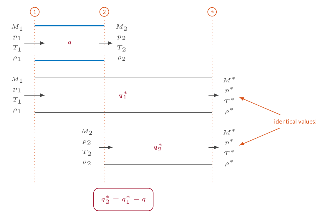
When heat is added to a one-dimensional flow, the Mach number will approach 1.0 (sonic flow). For an initially subsonic flow, the Mach number will increase until sonic conditions are reached and for an initially supersonic flow, added heat will reduce the Mach number until sonic conditions are reached. The heat addition for which sonic conditions are reached is denoted \(q^*\) and starred flow properties are flow properties at sonic conditions. The starred flow quantities are constants in a specific flow. When sonic conditions are reached, the flow is choked, and more heat cannot be added without changing the upstream flow conditions.
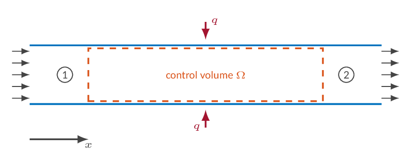
A typical problem is the two-station problem i.e., a problem where flow properties are known at one location in the flow and the flow properties in an upstream or downstream location should be calculated. This is done using the starred quantities as a reference state. The starred flow quantities are calculated based on the flow quantities in station 1. As the starred quantities are constants, they can be used together with the added heat to calculate the flow properties in station 2.
| flow property | adding heat to a subsonic flow | adding heat to a supersonic flow |
|---|---|---|
| density | decreases | increases |
| pressure | decreases | increases |
| velocity | increases | decreases |
| Mach number | increases | decreases |
| total pressure | decreases | decreases |
| entropy | increases | increases |
| total temperature | increases | increases |
More details can be found here:
| One-dimensional flow | (One-dimensional flow with heat addition) |
Friction is introduced by specifying a wall friction coefficient \(\bar{f}\). The wall friction coefficient is a dimensionless number and a typical value for turbulent flows is 0.005
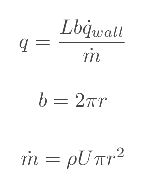
Added heat is introduced by specifying a heat source as either a wall heat flux \(\dot{q}_{wall}\ W/m^2\) or heat per unit mass \(q\ J/kg\). Heat per unit mass has to be complemented by a specified massflow.
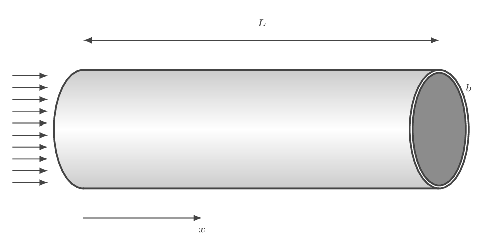
Heat per unit mass \((q)\) and wall heat flux \((\dot{q}_{wall})\) are related as follows
Specify friction coefficient and/or heat source term. If the heat source is specified as J/kg, massflow needs to be specified as well.
| wall friction \(\left(\bar{f}\right)\): | dimensionless, typical value ~0.005 | |||||
| wall heat \(\left(q\right)\): | ||||||
| massflow \(\left(\dot{m}\right)\): | ||||||
